Calculate the Intersection Between Two Densities

Usage

measureSimil(
  d1,
  d2,
  splits = 500,
  rawData = c(TRUE, TRUE),
  plot = TRUE,
  x_limit = "auto",
  colors = c("red", "blue", "gray"),
  ...
)

Arguments

d1, d2: Either two vectors of empirical (i.e., MCMC-produced) values OR a data.frame/matrix with columns x and y for values fitted to a density from which to calculate areas. If rawData is set to TRUE in any instance, the data must be placed in vectors and not multidimensional objects.
splits: A numerical argument controling the number of subdivisions of the intersection area for numerical integration
rawData: Are d1 and/or d2 raw data for which a density should be calculated? A vector of length two containing logical values indicating whenther any of the arguments d1 or d2 are raw data or whether the user is inputing already calculated densities (e.g., the output from the density, curve, or dDIST functions, or any two-dimension object with x and y values)
plot: Should a plot be produced?
x_limit: Whether to define the xlim form the min-max of the combined density x-values
colors: A vector of three colors, namely, color of the d1 density (e.g., the prior), color of the d2 density e.g., the posterior), and color of the intersection.
...: Further arguments to pass to the graphical functions such as lines and plot internally (e.g., main, xlim, ylim, xlab, ylab, etc.).

Value

A numeric vector with the value of the intersection between two densities. As a side effect, a plot is produced to an active (or new) graphical device.

Details

Similarity is measured as the overlapping portion between two densities. It has a value between 0 and 1. The values of the vector rawData determine the behavior of the function and therefore attention must be paid to their consistence with the nature of arguments d1 and d2. Despite the function was designed in order to allow to quantify similarity between the posterior and the prior, this can be used to quantify any overlap between two given densities and for any other purpose.

Examples

# \donttest{
# Set seed and colors to use in plots in the order: Prior, posterior, and intersection
set.seed(1985)
colors <- c("red", "blue", "lightgray")
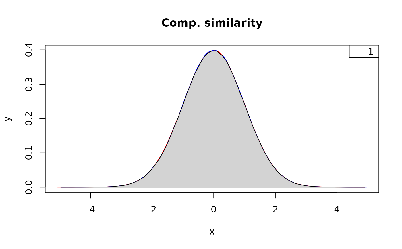
# Similarity between two identical distributions
below <- measureSimil(d1 = rnorm(1000000, mean = 0, 1),
                       d2 = rnorm(1000000, mean = 0, 1),
                       main = "Comp. similarity",
                       colors = colors)
legend(x = "topright", legend = round(below, digits = 2))

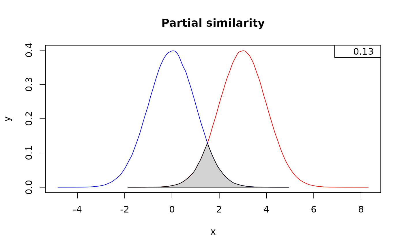
# Similarity in two distributions partially overlapping
below <- measureSimil(d1 = rnorm(1000000, mean = 3, 1),
                       d2 = rnorm(1000000, mean = 0, 1),
                       main = "Partial similarity",
                       colors = colors)
legend(x = "topright", legend = round(below, digits = 2))

# Similarity in two completely-different distributions
below <- measureSimil(d1 = rnorm(1000000, mean = 8, 1),
                       d2 = rnorm(1000000, mean = 0, 1),
                       main = "Comp. dissimilarity",
                       colors = colors)
legend(x = "topright", legend = round(below, digits = 2))

# Don't plot, just return the intersection
measureSimil(d1 = rnorm(1000000, mean = 3, 1),
              d2 = rnorm(1000000, mean = 0, 1),
              plot = FALSE)
#> [1] 0.1336534
# }